Introduction

Building a machine learning pipeline from scratch can be a daunting task, especially for those new to the field. This project post aims to simplify this process by providing a step-by-step guide to creating a comprehensive machine learning pipeline. We’ll cover everything from data preparation and model building to training, cross-validation, hyperparameter tuning, and visualization of results.

In this post, we’ll walk through the Python code necessary to build and evaluate machine learning models using libraries such as pandas, numpy, scikit-learn, PyTorch, and plotnine. We will start by importing the essential libraries and creating custom classes for modeling. These classes include a featureless baseline model, a neural network implemented in PyTorch, and a custom cross-validation class. We will then move on to data preparation, where we’ll preprocess datasets for training and testing.

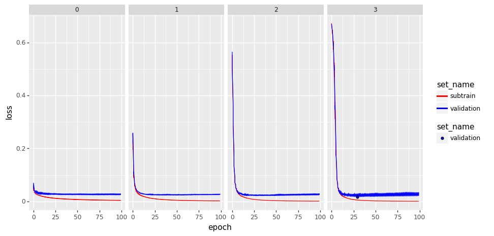
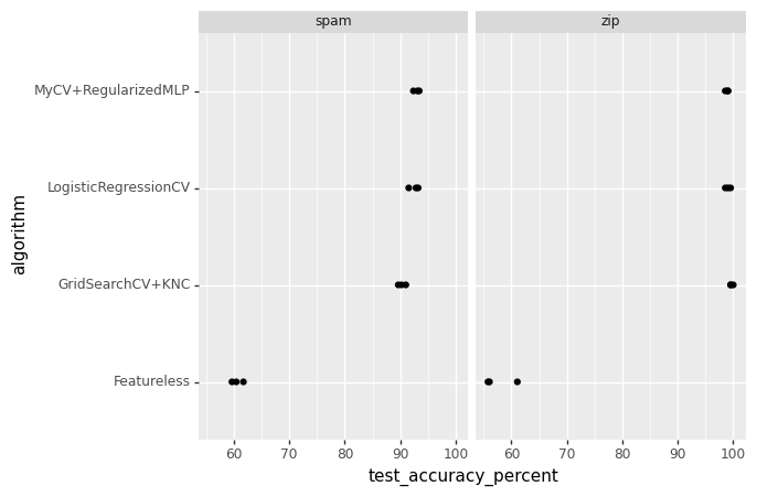
Following data preparation, we’ll train our models using various hyperparameters and generate diagnostic plots to visualize the results. Finally, we will apply our models to different datasets, comparing the performance of multiple algorithms to determine the best approach.

By the end of this post, you should have a clear understanding of how to build a robust machine learning pipeline, ready to be adapted and expanded for your specific needs. Let’s dive in!

Imports

The first step in any data science project is to import the necessary libraries. These libraries provide the tools for data manipulation, machine learning, and visualization.

import pandas as pd
import numpy as np
import torch
import plotnine as p9
from sklearn.model_selection import KFold
from sklearn.linear_model import LogisticRegressionCV
from sklearn.model_selection import GridSearchCV
from sklearn.neighbors import KNeighborsClassifier

Custom Classes

From the previous posts, we have created the FeaturelessModel class is a simple model that predicts the majority class in the training data.

The TorchModel class defines a neural network using PyTorch. It allows for flexible architecture by specifying the number of hidden layers and units per layer.

class TorchModel(torch.nn.Module):
    def __init__(self, n_hidden_layers, units_in_first_layer, units_per_hidden_layer=100):
        super(TorchModel, self).__init__()
        units_per_layer = [units_in_first_layer]
        for layer_i in range(n_hidden_layers):
            units_per_layer.append(units_per_hidden_layer)
        units_per_layer.append(1)
        seq_args = []
        for layer_i in range(len(units_per_layer)-1):
            units_in = units_per_layer[layer_i]
            units_out = units_per_layer[layer_i+1]
            seq_args.append(torch.nn.Linear(units_in, units_out))
            if layer_i != len(units_per_layer)-2:
                seq_args.append(torch.nn.ReLU())
        self.stack = torch.nn.Sequential(*seq_args)

    def forward(self, feature_mat):
        return self.stack(feature_mat)

The NumpyData class converts numpy arrays into a PyTorch dataset, making it easier to work with DataLoader for batch processing.

class NumpyData(torch.utils.data.Dataset):
    def __init__(self, features, labels):
        self.features = features
        self.labels = labels

    def __getitem__(self, item):
        return self.features[item, :], self.labels[item]

    def __len__(self):
        return len(self.labels)

The MyCV class handles cross-validation, iterating over parameter grids and tracking the best performing parameters.

class MyCV:
    def __init__(self, estimator, param_grid, cv):
        self.estimator = estimator
        self.param_grid = param_grid
        self.cv = cv

    def fit(self, X, y):
        self.train_features = X
        self.train_labels = y
        self.best_params_ = {}
        np.random.seed(1)
        fold_vec = np.random.randint(low=0, high=self.cv, size=self.train_labels.size)
        best_mean_accuracy = 0
        for param_dict in self.param_grid:
            for param_name, [param_value] in param_dict.items():
                setattr(self.estimator, param_name, param_value)
                accuracy_list = []
                loss_df_list = []
                for test_fold in range(self.cv):
                    is_set_dict = {"validation": fold_vec == test_fold, "subtrain": fold_vec != test_fold}
                    set_features = {set_name: self.train_features[is_set, :] for set_name, is_set in is_set_dict.items()}
                    set_labels = {set_name: self.train_labels[is_set] for set_name, is_set in is_set_dict.items()}
                    self.estimator.fit(X=set_features, y=set_labels)
                    predicted_labels = self.estimator.predict(X=set_features["validation"])
                    accuracy = np.mean(predicted_labels == set_labels["validation"])
                    loss_df_list.append(self.estimator.loss_df)
                    accuracy_list.append(accuracy)
                mean_accuracy = np.mean(accuracy_list)
                if mean_accuracy > best_mean_accuracy:
                    best_mean_accuracy = mean_accuracy
                    self.best_params_[param_name] = param_value
                    setattr(self.estimator, param_name, self.best_params_[param_name])

        self.loss_mean_df = pd.concat(loss_df_list)
        print(self.loss_mean_df)

    def predict(self, X):
        return self.estimator.predict(X)

The Regularized Multi-Layer Perceptron(RegularizedMLP) class builds and trains a neural network with regularization. It uses the TorchModel class to define the neural network architecture and the NumpyData class to convert numpy arrays into PyTorch datasets.

class RegularizedMLP:
    def __init__(self, max_epochs, batch_size, step_size, units_per_hidden_layer):
        self.max_epochs = max_epochs
        self.batch_size = batch_size
        self.step_size = step_size
        self.units_per_hidden_layer = units_per_hidden_layer
        self.loss_fun = torch.nn.BCEWithLogitsLoss()

    def fit(self, X, y):
        set_features = X
        set_labels = y
        subtrain_csv = NumpyData(set_features["subtrain"], set_labels["subtrain"])
        subtrain_dl = torch.utils.data.DataLoader(subtrain_csv, batch_size=self.batch_size, shuffle=True)
        loss_df_list = []
        for n_hidden_layers in range(self.hidden_layers):
            model = TorchModel(n_hidden_layers, set_features["subtrain"].shape[1])
            model.train()
            optimizer = torch.optim.SGD(model.parameters(), lr=0.2)
            for epoch in range(self.max_epochs):
                for batch_features, batch_labels in subtrain_dl:
                    pred_tensor = model(batch_features.float()).reshape(len(batch_labels.float()))
                    loss_tensor = self.loss_fun(pred_tensor, batch_labels.float())
                    optimizer.zero_grad()
                    loss_tensor.backward()
                    optimizer.step()
                for set_name in set_features:
                    feature_mat = set_features[set_name]
                    label_vec = set_labels[set_name]
                    feature_mat_tensor = torch.from_numpy(feature_mat.astype(np.float32))
                    label_vec_tensor = torch.from_numpy(label_vec.astype(np.float32))
                    pred_tensor = model(feature_mat_tensor.float()).reshape(len(label_vec_tensor.float()))
                    loss_tensor = self.loss_fun(pred_tensor, label_vec_tensor.float())
                    set_loss = loss_tensor.item()
                    loss_df_list.append(pd.DataFrame({
                        "n_hidden_layers": n_hidden_layers,
                        "set_name": set_name,
                        "loss": set_loss,
                        "epoch": epoch,
                    }, index=[0]))
        self.model = model
        self.loss_df = pd.concat(loss_df_list)

    def decision_function(self, X):
        self.model.eval()
        with torch.no_grad():
            return self.model(torch.Tensor(X)).numpy().ravel()

    def predict(self, X):
        return np.where(self.decision_function(X) > 0, 1, 0)

Data Preparation

Load and preprocess the datasets (spam and zip code data).

spam_df = pd.read_csv("./data/spam.data", header=None, sep=" ")
spam_features = spam_df.iloc[:, :-1].to_numpy()
spam_scaled_features = (spam_features - spam_features.mean(axis=0)) / spam_features.std(axis=0)
spam_labels = spam_df.iloc[:, -1].to_numpy()

zip_df = pd.read_csv("./data/zip.test.gz", header=None, sep=" ")
is01 = zip_df[0].isin([0, 1])
zip01_df = zip_df.loc[is01, :]
zip_features = zip01_df.loc[:, 1:].to_numpy()
zip_labels = zip01_df[0].to_numpy()
zip_scaled_features = (zip_features - zip_features.mean(axis=0)) / zip_features.std(axis=0)

data_dict = {
    "spam": (spam_scaled_features, spam_labels),
    "zip": (zip_features, zip_labels),
}

Hyperparameter Training and Diagnostic Plot

Train the models using cross-validation and generate diagnostic plots.

def hyperparameter_training_and_diagnostic_plot():
    for data_set, (input_mat, output_vec) in data_dict.items():
        param_dicts = [{'hidden_layers': [L]} for L in range(1, 5)]
        rmlp = RegularizedMLP(max_epochs=100, batch_size=200, step_size=0.2, units_per_hidden_layer=100)

        learner_instance = MyCV(estimator=rmlp, param_grid=param_dicts, cv=2)
        learner_instance.fit(input_mat, output_vec)
        print(learner_instance.best_params_)

        loss_df = learner_instance.loss_mean_df
        loss_df.index = range(len(loss_df))

        def get_min(series_obj):
            return series_obj.index[series_obj.argmin()]

        rows_to_plot = loss_df.groupby(["n_hidden_layers", "set_name"])["loss"].apply(get_min)
        layers_plot_data = loss_df.iloc[rows_to_plot, :]

        set_colors = {"subtrain": "red", "validation": "blue"}
        gg = p9.ggplot() +\
            p9.facet_grid(". ~ set_name") +\
            p9.scale_color_manual(values=set_colors) +\
            p9.geom_line(
                p9.aes(
                    x="epoch",
                    y="loss",
                    color="n_hidden_layers"
                ),
                data=loss_df) +\
            p9.geom_point(
                p9.aes(
                    x="epoch",
                    y="loss",
                    color="n_hidden_layers"
                ),
                data=layers_plot_data)
        gg.save(f"./11_regularization/{data_set}_03.png", width=10, height=5)

        set_colors = {1: "red", 2: "green", 3: "blue", 4: "orange"}
        gg = p9.ggplot() +\
            p9.facet_grid(". ~ set_name") +\
            p9.scale_color_manual(values=set_colors) +\
            p9.geom_line(
                p9.aes(
                    x="epoch",
                    y="loss",
                    color="n_hidden_layers"
                ),
                data=loss_df) +\
            p9.geom_point(
                p9.aes(
                    x="epoch",
                    y="loss",
                    color="n_hidden_layers"
                ),
                data=layers_plot_data)
        gg.save(f"./{data_set}_01.png", width=10, height=5)

        validation_df = loss_df.query("set_name=='validation'")
        min_i = validation_df.loss.argmin()
        min_row = pd.DataFrame(dict(validation_df.iloc[min_i, :]), index=[0])
        gg = p9.ggplot() +\
            p9.facet_grid(". ~ n_hidden_layers") +\
            p9.scale_color_manual(values=set_colors) +\
            p9.scale_fill_manual(values=set_colors) +\
            p9.geom_line(
                p9.aes(
                    x="epoch",
                    y="loss",
                    color="set_name"
                ),
                data=loss_df) +\
            p9.geom_point(
                p9.aes(
                    x="epoch",
                    y="loss",
                    fill="set_name"
                ),
                color="black",
                data=min_row)
        gg.save(f"./{data_set}_02.png", width=10, height=5)

Experiments and Application

This function applies the model to different datasets and compares the performance of various algorithms.

def experiments_and_application():
    test_acc_df_list = []
    for data_set, (input_mat, output_vec) in data_dict.items():
        k_fold = KFold(n_splits=3, shuffle=True, random_state=1)
        for fold_id, indices in enumerate(k_fold.split(input_mat)):
            index_dict = dict(zip(["train", "test"], indices))

            set_data_dict = {}
            for set_name, index_vec in index_dict.items():
                set_data_dict[set_name] = {
                    "X": input_mat[index_vec],
                    "y": output_vec[index_vec]
                }

            rmlp = RegularizedMLP(
                max_epochs=100,
                batch_size=200,
                step_size=0.2,
                units_per_hidden_layer=100,
            )
            learner_instance = MyCV(estimator=rmlp, param_grid=[
                                    {'hidden_layers': [L]} for L in range(1, 5)], cv=2)
            learner_instance.fit(**set_data_dict["train"])

            logistic_reg_cv = LogisticRegressionCV(max_iter=1000)
            logistic_reg_cv.fit(**set_data_dict["train"])

            grid_search_cv = GridSearchCV(estimator=KNeighborsClassifier(), param_grid=[
                                          {'n_neighbors': [x]} for x in range(1, 21)], cv=5)
            grid_search_cv.fit(**set_data_dict["train"])

            featureless = Featureless()
            featureless.fit(set_data_dict["train"]['y'])

            test_data_x = set_data_dict["test"]['X']
            test_data_y = set_data_dict["test"]['y']

            pred_dict = {
                "LogisticRegressionCV": logistic_reg_cv.predict(test_data_x),
                "Featureless": featureless.predict(test_data_x),
                "GridSearchCV+KNC": grid_search_cv.predict(test_data_x),
                "MyCV+RegularizedMLP": learner_instance.predict(set_data_dict["test"]['X']),
            }
            for algorithm, pred_vec in pred_dict.items():
                test_acc_dict = {
                    "test_accuracy_percent": (pred_vec == test_data_y).mean()*100,
                    "data_set": data_set,
                    "fold_id": fold_id,
                    "algorithm": algorithm
                }
                test_acc_df_list.append(pd.DataFrame(test_acc_dict, index=[0]))

    test_acc_df = pd.concat(test_acc_df_list)
    print(test_acc_df)

    gg = p9.ggplot() +\
        p9.geom_point(
            p9.aes(
                x="test_accuracy_percent",
                y="algorithm"
            ),
            data=test_acc_df) +\
        p9.facet_wrap("data_set")
    gg.save("./p8_accuracy_facetted.png")

Conclusion

This pipeline integrates various components of machine learning workflow, including data preparation, model building, training, hyperparameter tuning, and result visualization. The use of custom classes and functions allows for flexibility and reusability in different machine learning scenarios. This project post aims to provide a comprehensive overview and a practical implementation guide for building a machine learning pipeline from scratch.