Custom ML Algorithms
Evaluating custom ML models on spam and zip benchmark datasets.
Introduction
This project involves building and evaluating various machine learning models to classify the zip and spam datasets. The steps include data preprocessing, model training, hyperparameter tuning, and performance evaluation. The code is implemented in Python using libraries such as pandas, numpy, plotnine, and scikit-learn.
import pandas as pd
import numpy as np
import plotnine as p9
from sklearn.model_selection import KFold
from sklearn.linear_model import LogisticRegression
from sklearn.pipeline import make_pipeline
from sklearn.preprocessing import StandardScaler
from sklearn.model_selection import GridSearchCV
from sklearn.neighbors import KNeighborsClassifier
Model Classes
We define custom classes for different models and utilities.
Featureless: A baseline model that predicts the most frequent label.
class Featureless:
    def fit(self, y):
        train_labels = y
        train_label_counts = pd.Series(train_labels).value_counts()
        self.featureless_pred_label = train_label_counts.idxmax()

    def predict(self, X):
        test_features = X
        test_nrow, test_ncol = test_features.shape
        return np.repeat(self.featureless_pred_label, test_nrow)
MyKNN: A custom K-Nearest Neighbors implementation.
class MyKNN:
    def __init__(self, n_neighbors=5):
        self.n_neighbors = n_neighbors

    def fit(self, X, y):
        self.train_features = X
        self.train_labels = y

    def predict(self, X):
        predicted_labels = []
        for test_i in range(X.shape[0]):
            test_i_features = X[test_i, :]
            diff_mat = self.train_features - test_i_features
            squared_diff_mat = diff_mat ** 2
            squared_diff_mat.sum(axis=0)
            distance_vec = squared_diff_mat.sum(axis=1)
            sorted_indices = distance_vec.argsort()
            nearest_indices = sorted_indices[:self.n_neighbors]
            nearest_labels = self.train_labels[nearest_indices]
            predicted_label = np.argmax(np.bincount(nearest_labels))
            predicted_labels.append(predicted_label)

        predicted_labels = np.array(predicted_labels)
        return predicted_labels
MyCV: A custom cross-validation class for hyperparameter tuning.
class MyCV:
    def __init__(self, estimator, param_grid, cv):
        self.estimator = estimator
        self.param_grid = param_grid
        self.cv = cv

    def fit(self, X, y):
        self.train_features = X
        self.train_labels = y
        self.best_params_ = {}
        np.random.seed(1)
        fold_vec = np.random.randint(low=0, high=self.cv, size=self.train_labels.size)
        best_mean_accuracy = 0
        for param_dict in self.param_grid:
            for param_name, [param_value] in param_dict.items():
                setattr(self.estimator, param_name, param_value)
                accuracy_list = []
                for test_fold in range(self.cv):
                    is_set_dict = {
                        "validation": fold_vec == test_fold,
                        "subtrain": fold_vec != test_fold,
                    }
                    set_features = {
                        set_name: self.train_features[is_set, :]
                        for set_name, is_set in is_set_dict.items()
                    }
                    set_labels = {
                        set_name: self.train_labels[is_set]
                        for set_name, is_set in is_set_dict.items()
                    }
                    self.estimator.fit(X=set_features["subtrain"], y=set_labels["subtrain"])
                    predicted_labels = self.estimator.predict(X=set_features["validation"])
                    accuracy = np.mean(predicted_labels == set_labels["validation"])
                    accuracy_list.append(accuracy)
                mean_accuracy = np.mean(accuracy_list)
                if mean_accuracy > best_mean_accuracy:
                    best_mean_accuracy = mean_accuracy
                    self.best_params_[param_name] = param_value
            setattr(self.estimator, param_name, self.best_params_[param_name])

    def predict(self, X):
        return self.estimator.predict(X)
MyPipeline: A custom pipeline to sequentially apply a list of transforms and a final estimator.
class MyPipeline:
    def __init__(self, steps):
        self.steps = steps

    def fit(self, X, y):
        for step in self.steps:
            if hasattr(step, "transform"):
                X = step.transform(X)
            else:
                X = step.fit(X, y)

    def predict(self, X):
        for step in self.steps:
            if hasattr(step, "transform"):
                X = step.transform(X)
            else:
                X = step.predict(X)
        return X

def make_my_pipeline(*steps):
    return MyPipeline(steps)
MyStandardScaler: A custom standard scaler for feature scaling.
class MyStandardScaler:
    def fit(self, X):
        self.mean = X.mean(axis=0)
        self.std = X.std(axis=0)

    def transform(self, X):
        self.fit(X)
        for row in range(X.shape[0]):
            for col in range(X.shape[1]):
                if self.std[col] != 0:
                    X[row, col] = (X[row, col] - self.mean[col]) / self.std[col]
        return X

    def fit_transform(self, X, y):
        self.fit(X)
        return self.transform(X)
Data Loading
Load the zip and spam datasets.
# Load zip data
zip_df = pd.read_csv("./data/zip.test.gz", header=None, sep=" ")
is01 = zip_df[0].isin([0, 1])
zip01_df = zip_df.loc[is01, :]
zip_features = zip01_df.loc[:, 1:].to_numpy()
zip_labels = zip01_df[0].to_numpy()

# Load the spam data
spam_df = pd.read_csv("./data/spam.data", sep=" ", header=None)
spam_features = spam_df.iloc[:, :-1].to_numpy()
spam_labels = spam_df.iloc[:, -1].to_numpy()

data_dict = {
    "zip": (zip_features, zip_labels),
    "spam": (spam_features, spam_labels),
    "spam_scaled": (MyStandardScaler().fit_transform(spam_features, spam_labels), spam_labels),
}
Model Training and Evaluation
Different models are trained and evaluated using cross-validation. Models include logistic regression, KNN with cross-validation, and featureless classifier. Hyperparameter tuning is performed for KNN using MyCV and GridSearchCV.
test_acc_df_list = []

for data_set, (input_mat, output_vec) in data_dict.items():
    k_fold = KFold(n_splits=3, shuffle=True, random_state=1)
    for fold_id, indices in enumerate(k_fold.split(input_mat)):
        index_dict = dict(zip(["train", "test"], indices))
        param_dicts = [{'n_neighbors': [x]} for x in range(1, 21)]

        set_data_dict = {}
        for set_name, index_vec in index_dict.items():
            set_data_dict[set_name] = {
                "X": input_mat[index_vec],
                "y": output_vec[index_vec]
            }

        pipe = make_pipeline(StandardScaler(), LogisticRegression(max_iter=1000))
        pipe.fit(**set_data_dict["train"])

        my_cv = MyCV(estimator=MyKNN(), param_grid=param_dicts, cv=5)
        my_cv.fit(**set_data_dict["train"])

        my_cv_scaled = make_my_pipeline(MyStandardScaler(),
        MyCV(estimator=MyKNN(), param_grid=param_dicts, cv=5))
        my_cv_scaled.fit(**set_data_dict["train"])

        grid_search_cv_scaled = make_pipeline(StandardScaler(),
        GridSearchCV(estimator=KNeighborsClassifier(), param_grid=param_dicts, cv=5))
        grid_search_cv_scaled.fit(**set_data_dict["train"])

        featureless = Featureless()
        featureless.fit(set_data_dict["train"]['y'])

        test_data_x = set_data_dict["test"]['X']
        test_data_y = set_data_dict["test"]['y']

        pred_dict = {
            "linear_model": pipe.predict(test_data_x),
            "featureless": featureless.predict(test_data_x),
            "MyCV+MyKNN": my_cv.predict(test_data_x),
            "MyCV+MyKNN+Scaled": my_cv_scaled.predict(test_data_x),
            "GridSearchCV+KNNC+Scaled": grid_search_cv_scaled.predict(test_data_x),
        }
        for algorithm, pred_vec in pred_dict.items():
            test_acc_dict = {
                "test_accuracy_percent": (pred_vec == test_data_y).mean() * 100,
                "data_set": data_set,
                "fold_id": fold_id,
                "algorithm": algorithm
            }
            test_acc_df_list.append(pd.DataFrame(test_acc_dict, index=[0]))

test_acc_df = pd.concat(test_acc_df_list)
print(test_acc_df)
Performance Visualization
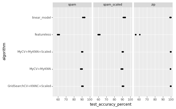
Create a facetted plot to visualize the performance of different models on the zip and spam datasets.
# make a facetted plot with one panel per image
gg = p9.ggplot() +\
    p9.geom_point(
        p9.aes(
            x="test_accuracy_percent",
            y="algorithm"
        ),
        data=test_acc_df) +\
    p9.facet_wrap("data_set")
gg.save("./p6_accuracy_facetted.png")

Interpretation
The scatter plot provides a comparative analysis of the test accuracy percentages achieved by three different algorithms on three datasets. The algorithms are GridSearchCV+KNNC+Scaled, MyCV+MyKNN+Scaled, and MyCV+MyKNN and the datasets are labeled as spam, spam_scaled and zip.
Axes Description
- X-Axis (test_accuracy_percent): Represents the accuracy percentage achieved by the algorithms, ranging from 60 to 100.
- Y-Axis (algorithm): Lists the algorithms evaluated in the analysis.
Data Points
- Each algorithm has one data point per dataset category, indicating the performance of that particular algorithm on the given dataset.
- The categories
spamandspam_scaledlikely represent the original and scaled versions of the spam dataset, whileziprepresents a separate dataset.
Observations
- The
GridSearchCV+KNNC+Scaledalgorithm shows high accuracy across all datasets, with particularly notable performance on thespam_scaleddataset. - The
MyCV+MyKNN+Scaledalgorithm also performs well, especially on the scaled datasets, suggesting that scaling improves its accuracy. - The
MyCV+MyKNNalgorithm without scaling shows lower accuracy compared to its scaled counterpart, highlighting the impact of feature scaling on model performance.
Conclusion
The scatter plot effectively demonstrates the importance of data preprocessing, such as scaling, and its impact on the performance of machine learning algorithms. It also allows for a quick visual comparison between different modeling approaches and their effectiveness across various types of data.